In-class_Exercise 2

Overview

In this exercise, we are to find out if functionally similar water points positively co-occur in Nigeria.

Getting Started

In the code chunk below, p_load() of pacman package is used to install and load the following R packages into R environment:

sf
tidyverse
tmap
spdep
funModeling, to be used for rapid Exploratory Data Analysis

pacman::p_load(sf, tidyverse, tmap, spdep, funModeling)

Importing Geospatial Data

In this in-class exercise, two geospatial data sets will be used:

geo_export
nga_admbnda_adm2_osgof_20190417

Importing water point geospatial data

First, we are going to import the water point geospatial data (i.e. geo_export) by using the code chunk below.

wp <- st_read(dsn = "rawdata",
              layer = "geo_export",
              crs = 4326) %>%
  filter(clean_coun == "Nigeria")

Things to learn from the code chunk above:

st_read() of sf package is used to import geo_export shapefile into R environment and save the imported geospatial data into simple feature data table.
filter() of dplyr package is used to extract water point records of Nigeria only.

Note: Avoid performing transformation if you plan to use st_intersects() of sf package in the later stage of the geoprocessing. This is because st_intersects() only works correctly if the geospatial data are in geographic coordinate system (i.e wgs84).

Next, write_rds() of readr package is used to save the extracted sf data table (i.e. wp) into an output file in rds data format. The output file is called wp_nga.rds and it is saved in rawdata sub-folder, which will not be uploaded to Git.

wp_nga <- write_rds(wp,
                    "rawdata/wp_nga.rds")

Importing Nigeria LGA boundary data

Now, we are going to import the Local Government Area (LGA) boundary data into R environment by using the code chunk below.

nga <- st_read(dsn = "data",
               layer = "nga_admbnda_adm2_osgof_20190417",
               crs = 4326)

Reading layer `nga_admbnda_adm2_osgof_20190417' from data source 
  `C:\Jacobche\ISSS624\In-class_Ex\data' using driver `ESRI Shapefile'
Simple feature collection with 774 features and 16 fields
Geometry type: MULTIPOLYGON
Dimension:     XY
Bounding box:  xmin: 2.668534 ymin: 4.273007 xmax: 14.67882 ymax: 13.89442
Geodetic CRS:  WGS 84

Thing to learn from the code chunk above.

st_read() of sf package is used to import nga_admbnda_adm2_osgof_20190417 shapefile into R environment and save the imported geospatial data into simple feature data table.

Data Wrangling

Recoding NA values into string

In the code chunk below, replace_na() is used to recode all the NA values in status_cle field into Unknown.

wp_nga <- read_rds("rawdata/wp_nga.rds") %>%
  mutate(status_cle = replace_na(status_cle, "Unknown"))

Exploratory Data Analysis

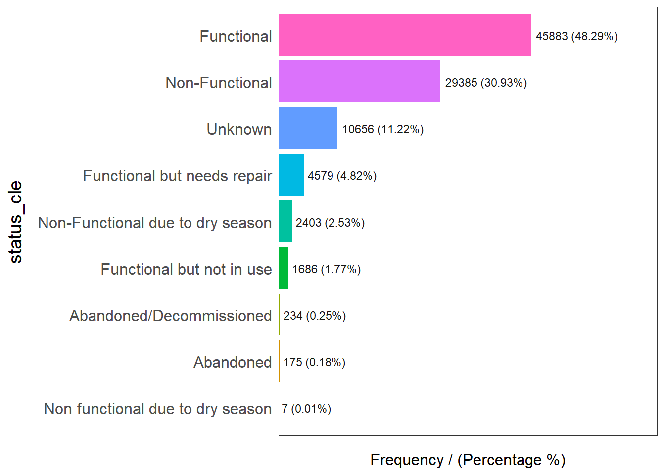
In the code chunk below, freq() of funModeling package is used to display the distribution of status_cle field in wp_nga.

freq(data=wp_nga, 
     input = 'status_cle')

                        status_cle frequency percentage cumulative_perc
1                       Functional     45883      48.29           48.29
2                   Non-Functional     29385      30.93           79.22
3                          Unknown     10656      11.22           90.44
4      Functional but needs repair      4579       4.82           95.26
5 Non-Functional due to dry season      2403       2.53           97.79
6        Functional but not in use      1686       1.77           99.56
7         Abandoned/Decommissioned       234       0.25           99.81
8                        Abandoned       175       0.18           99.99
9 Non functional due to dry season         7       0.01          100.00

Extracting Water Point Data

In this section, we will extract the water point records by using classes in status_cle field.

Extracting functional water point

In the code chunk below, filter() of dplyr is used to select functional water points.

wpt_functional <- wp_nga %>%
  filter(status_cle %in%
           c("Functional", 
             "Functional but not in use",
             "Functional but needs repair"))

Exploratory Data Analysis (functional)

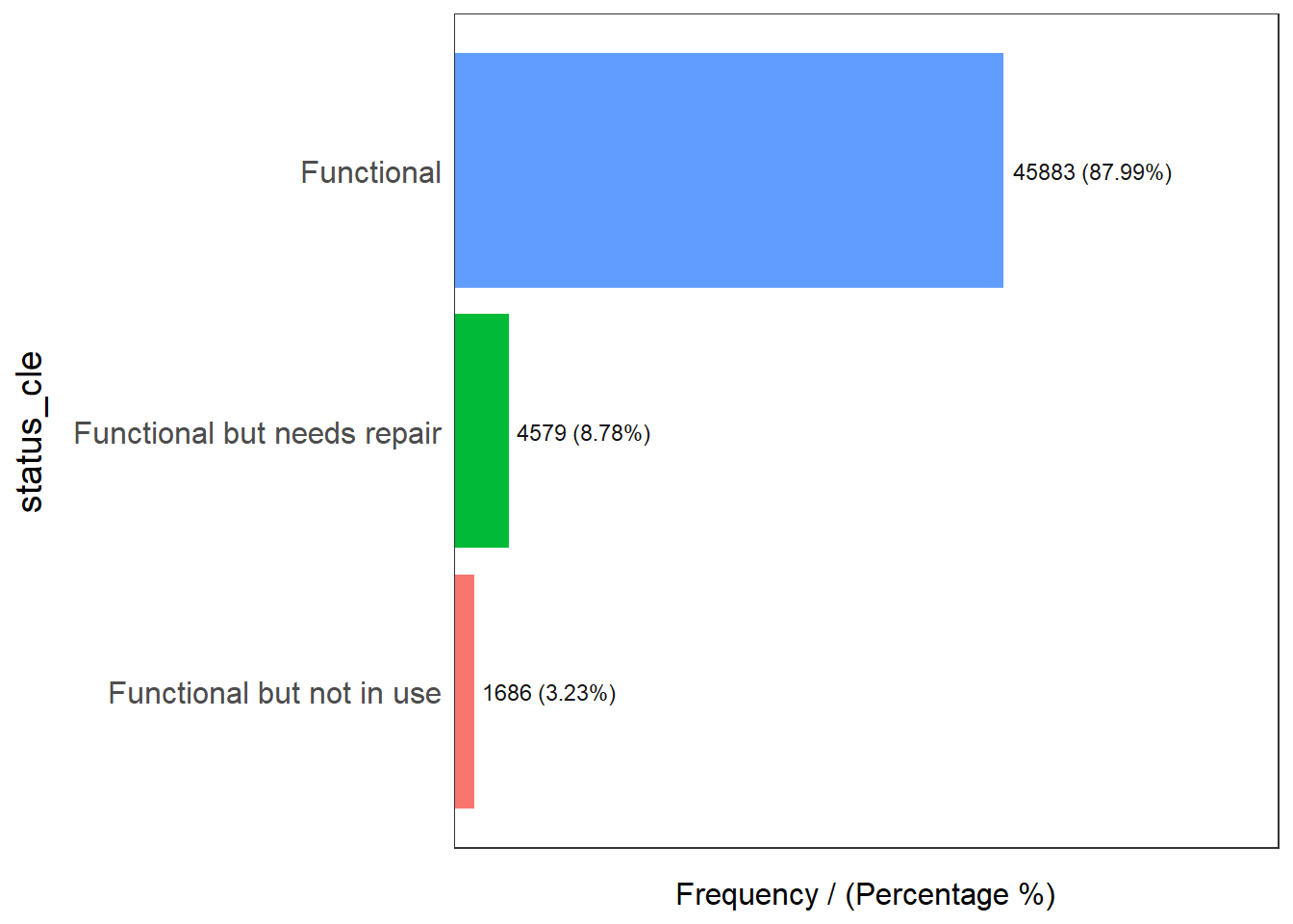
In the code chunk below, freq() of funModeling package is used to display the distribution of status_cle field in wpt_functional.

freq(data=wpt_functional, 
     input = 'status_cle')

                   status_cle frequency percentage cumulative_perc
1                  Functional     45883      87.99           87.99
2 Functional but needs repair      4579       8.78           96.77
3   Functional but not in use      1686       3.23          100.00

Extracting non-functional water point

In the code chunk below, filter() of dplyr is used to select non-functional water points.

wpt_nonfunctional <- wp_nga %>%
  filter(status_cle %in%
           c("Abandoned/Decommissioned", 
             "Abandoned",
             "Non-Functional",
             "Non functional due to dry season",
             "Non-Functional due to dry season"))

Exploratory Data Analysis (non-functional)

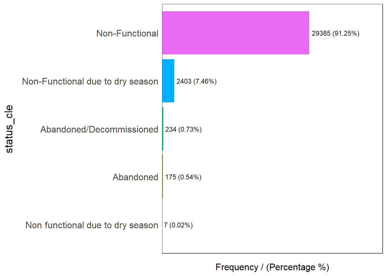
In the code chunk below, freq() of funModeling package is used to display the distribution of status_cle field in wpt_nonfunctional.

freq(data=wpt_nonfunctional, 
     input = 'status_cle')

                        status_cle frequency percentage cumulative_perc
1                   Non-Functional     29385      91.25           91.25
2 Non-Functional due to dry season      2403       7.46           98.71
3         Abandoned/Decommissioned       234       0.73           99.44
4                        Abandoned       175       0.54           99.98
5 Non functional due to dry season         7       0.02          100.00

Extracting water point with Unknown class

In the code chunk below, filter() of dplyr is used to select water points with unknown status.

wpt_unknown <- wp_nga %>%
  filter(status_cle == "Unknown")

Performing Point-in-Polygon Count

The code chunk below performs two operations at one go. Firstly, identify water points located inside each LGA by using st_intersects(). Next, length() of Base R is used to calculate numbers of water points that fall inside each LGA.

nga_wp <- nga %>% 
  mutate(`total wpt` = lengths(
    st_intersects(nga, wp_nga))) %>%
  mutate(`wpt functional` = lengths(
    st_intersects(nga, wpt_functional))) %>%
  mutate(`wpt non-functional` = lengths(
    st_intersects(nga, wpt_nonfunctional))) %>%
  mutate(`wpt unknown` = lengths(
    st_intersects(nga, wpt_unknown)))

Saving the Analytical Data Table

The code chunk below computes the proportion of functional and non-functional water point at LGA level.

nga_wp <- nga_wp %>%
  mutate(pct_functional = `wpt functional`/`total wpt`) %>%
  mutate(`pct_non-functional` = `wpt non-functional`/`total wpt`) %>%
  select(3:4, 9:10, 18:23)

Things to learn from the code chunk above:

mutate() of dplyr package is used to derive two fields namely pct_functional and pct_non-functional.
to keep the file size small, select() of dplyr is used to retain only fields 3, 4, 9, 10, 18, 19, 20, 21, 22 and 23.

Now, we have the tidy sf data table for subsequent analysis. We will save the sf data table into rds format.

write_rds(nga_wp, "data/nga_wp.rds")

Visualising the spatial distribution of water points

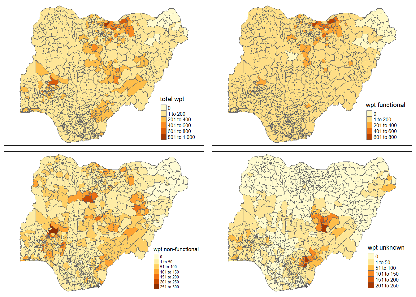
The code below uses qtm() of tmap package to plot side-by-side choropleth maps showing various water points distribution by LGA levels in Nigeria.

nga_wp <- read_rds("data/nga_wp.rds")
total <- qtm(nga_wp, "total wpt") +
  tm_layout(scale = 0.7)
wp_functional <- qtm(nga_wp, "wpt functional")+
  tm_layout(scale = 0.7)
wp_nonfunctional <- qtm(nga_wp, "wpt non-functional")+
  tm_layout(scale = 0.6)
unknown <- qtm(nga_wp, "wpt unknown")+
  tm_layout(scale = 0.7)

tmap_arrange(total, wp_functional, wp_nonfunctional, unknown, nrow=2, ncol=2)