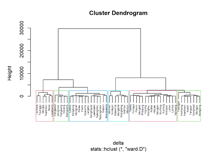
nongeo_cluster <- hclustgeo(proxmat)
plot(nongeo_cluster, cex = 0.5)
rect.hclust(nongeo_cluster,
            k = 6,
border = 2:5)In-class Exercise 3
Spatially Constrained Clustering: ClustGeo Method
To continue from Hands-on Exercise 3, in this section we will use functions provided by ClustGeo package to perform non-spatially constrained hierarchical cluster analysis and spatially constrained cluster analysis.
Ward-like hierarchical clustering: ClustGeo
ClustGeo package provides function called hclustgeo() to perform a typical Ward-like hierarchical clustering just like hclust() we used in previous section.
To perform non-spatially constrained hierarchical clustering, we only need to provide the function a dissimilarity matrix as shown in the code chunk below.
Note that the dissimilarity matrix must be an object of class dist, i.e. an object obtained with the function dist(). For sample code chunk, please refer to the session on Computing proximity matrix.
Mapping the clusters formed
Similarly, we can plot the clusters on a categorical area shaded map by using the steps we used in the session on Mapping the clusters formed.
groups <- as.factor(cutree(nongeo_cluster, k=6))shan_sf_ngeo_cluster <- cbind(shan_sf, as.matrix(groups)) %>%
rename(`CLUSTER` = `as.matrix.groups.`)qtm(shan_sf_ngeo_cluster, "CLUSTER")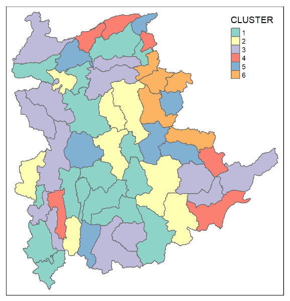
Spatially Constrained Hierarchical Clustering
Before we can perform spatially constrained hierarchical clustering, a spatial distance matrix will be derived by using st_distance() of sf package.
dist <- st_distance(shan_sf, shan_sf)
distmat <- as.dist(dist)
Notice that as.dist() is used to convert the data frame into matrix.
Next, choicealpha() will be used to determine a suitable value for the mixing parameter alpha as shown in the code chunk below.
cr <- choicealpha(proxmat, distmat, range.alpha = seq(0, 1, 0.1), K=6, graph = TRUE)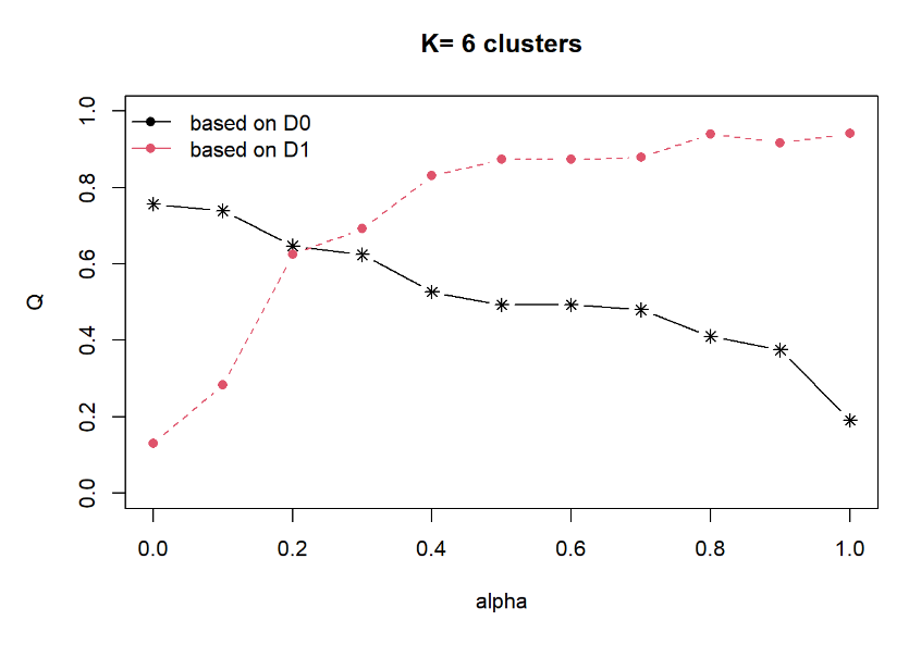
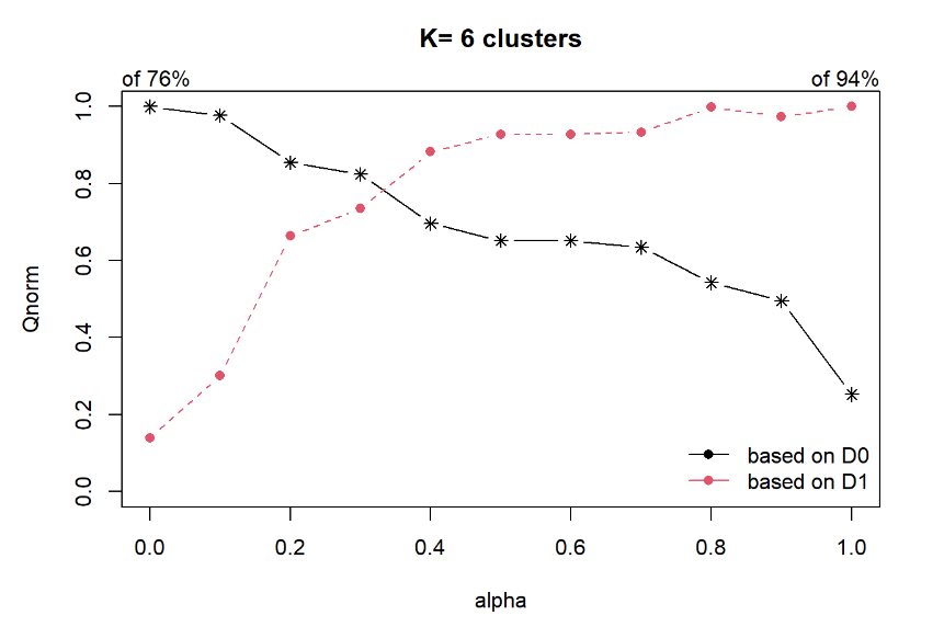 With reference to the graphs above, alpha = 0.3 will be used as shown in the code chunk below.
clustG <- hclustgeo(proxmat, distmat, alpha = 0.3)Next, cutree() is used to derive the cluster object.
groups <- as.factor(cutree(clustG, k=6))We will then join back the group list with shan_sf polygon feature data frame by using the code chunk below.
shan_sf_Gcluster <- cbind(shan_sf, as.matrix(groups)) %>%
  rename(`CLUSTER` = `as.matrix.groups.`)
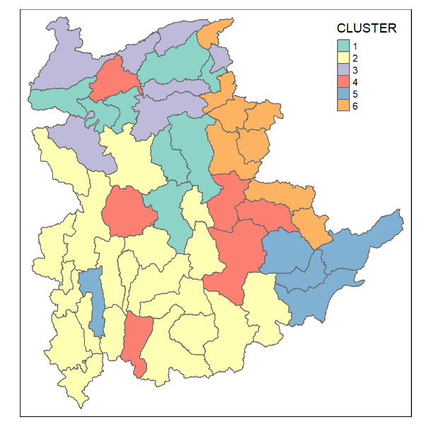
We can now plot the map of the newly delineated spatially constrained clusters.
qtm(shan_sf_Gcluster, "CLUSTER")